Performing Zonal Statistics on GHS-OBAT Building Data: A Case Study in Amsterdam¶

by Samapriya Roy

This tutorial demonstrates a scalable workflow for performing zonal statistics on the Global Human Settlement - Open Buildings Attribute Table (GHS-OBAT) dataset using custom administrative boundaries. By leveraging the GHS-OBAT's rich building-level attributes, we can derive meaningful insights at a local scale.

The analysis uses two primary datasets:

GHS-OBAT: A feature collection providing building footprints for the Netherlands, enriched with attributes like construction epoch and height from the Global Human Settlement Layer (GHSL).
Amsterdam Neighborhoods: A feature collection of polygons defining the zones for our statistical analysis.

The methodology involves loading and filtering the data, creating a function to calculate statistics per zone, applying this function across all zones using .map(), and visualizing the results with both choropleth maps and ui.Chart.

1. Data Preparation and Filtering¶

The first step in any analysis is to prepare the input data. This involves loading the relevant collections, spatially filtering the GHS-OBAT data to our area of interest (AOI) for efficiency, and cleaning the data to ensure analytical integrity.

Loading Datasets: We load the GHS-OBAT collection for the Netherlands (NLD) and the Amsterdam neighborhood boundaries.
Spatial Filtering: We apply .filterBounds() to the GHS-OBAT collection. This is a critical performance optimization that reduces the dataset to only those features that intersect with the neighborhood boundaries before any further processing.
Attribute Cleaning: We filter the resulting collection to exclude buildings with null or invalid values for height and epoch, which are the primary attributes for this analysis.

// Load the datasets
var amsterdam_neighbourhoods = ee.FeatureCollection("projects/sat-io/open-datasets/INSIDE-AIRBNB/amsterdam_neighbourhoods");
var GHS_OBAT_NLD = ee.FeatureCollection("projects/sat-io/open-datasets/JRC/GHS-OBAT/GHS_OBAT_GPKG_NLD_E2020_R2024A_V1_0");

// Spatially filter buildings to the Amsterdam area
var amsterdam_buildings = GHS_OBAT_NLD.filterBounds(amsterdam_neighbourhoods);

// Clean the data to ensure valid attributes for analysis
var valid_buildings = amsterdam_buildings.filter(ee.Filter.and(
  ee.Filter.neq('height', null),
  ee.Filter.neq('epoch', null),
  ee.Filter.gt('height', 0),
  ee.Filter.gte('epoch', 0)
));

print('Total valid buildings in Amsterdam area:', valid_buildings.size());

2. Implementing Zonal Statistics with a Mapped Function¶

The core of this analysis is to calculate statistics for each neighborhood polygon. The most efficient way to accomplish this in Earth Engine is to define a function that processes a single feature and then apply it to the entire collection using .map().

Our calculateNeighborhoodStats function executes the following steps for each neighborhood:

Filters the valid_buildings collection to the geometry of the input neighborhood.
Calculates aggregate statistics (e.g., mean, min, max) for numeric properties like height and epoch using aggregate_stats.
Performs categorical counts for distributions, such as the number of buildings within each construction epoch and within custom-defined height ranges. This requires a series of .filter().size() calls.
Attaches the results as new properties to the input neighborhood feature using .set(). Note the practice of adding both raw property names (e.g., epoch_1) and descriptive, chart-friendly names (e.g., 'Before 1980') for downstream flexibility.

This function is then mapped over the amsterdam_neighbourhoods collection, executing the entire statistical analysis as a single server-side operation.

// Function to calculate zonal statistics for each neighborhood
function calculateNeighborhoodStats(neighborhood) {
  var neighborhood_buildings = valid_buildings.filterBounds(neighborhood.geometry());

  // Calculate aggregate and categorical statistics
  var building_count = neighborhood_buildings.size();
  var height_stats = neighborhood_buildings.aggregate_stats('height');
  var epoch_1_count = neighborhood_buildings.filter(ee.Filter.eq('epoch', 1)).size();
  // ... (additional counts for other epochs and height ranges)

  // Add all statistics as properties to the neighborhood feature
  return neighborhood
    .set('building_count', building_count)
    .set('height_mean', height_stats.get('mean'))
    // ... (other aggregate stats)
    // Set chart-friendly property names
    .set('Before 1980', epoch_1_count)
    .set('1980-1990', neighborhood_buildings.filter(ee.Filter.eq('epoch', 2)).size());
    // ... (other descriptive properties)
}

// Apply the function to every neighborhood feature
var neighborhoods_with_stats = amsterdam_neighbourhoods.map(calculateNeighborhoodStats);
print('Sample neighborhood with enriched statistics:', neighborhoods_with_stats.first());

3. Visualization and Interpretation¶

With the neighborhoods_with_stats collection now enriched with our calculated data, we can visualize the results to identify spatial patterns and trends.

Choropleth Maps¶

Choropleth maps are effective for visualizing the spatial distribution of a variable. We can style the neighborhood polygons based on a calculated property, such as 'building_count' or 'height_mean'. The fillColor parameter is dynamically assigned from the feature property, and a palette defines the color ramp.

// Create a choropleth map for mean building height
Map.addLayer(
  neighborhoods_with_stats,
  {
    color: 'black',
    width: 1,
    fillColor: 'height_mean', // Use the calculated property
    palette: ['#fee5d9', '#fcbba1', '#fc9272', '#fb6a4a', '#de2d26', '#a50f15'],
    min: 3,
    max: 15
  },
  'Mean Building Height by Neighborhood',
  false // Layer initially hidden
);

Interactive Charts¶

For comparing distributions across multiple categories and neighborhoods, ui.Chart is the ideal tool. By using ui.Chart.feature.byFeature, we can create stacked column charts to explore the building stock's composition.

Crucially, we provide the array of chart-friendly property names we created earlier (e.g., 'Before 1980') as the yProperties. Earth Engine uses these strings directly as labels in the chart's legend, producing a clear and interpretable visualization without requiring manual label overrides in the chart options.

// Height distribution chart
var heightChart = ui.Chart.feature.byFeature({
  features: neighborhoods_with_stats.limit(15),
  xProperty: 'neighbourh',
  // Use the descriptive property names for the y-axis
  yProperties: ['0-5m', '5-10m', '10-20m', '20m+']
})
.setChartType('ColumnChart')
.setOptions({
  title: 'Building Height Distribution by Neighborhood (Top 15)',
  hAxis: {title: 'Neighborhood'},
  vAxis: {title: 'Number of Buildings'},
  isStacked: true,
  legend: {position: 'right'}
});
print(heightChart);

// Epoch distribution chart
var epochChart = ui.Chart.feature.byFeature({
  features: neighborhoods_with_stats.limit(15),
  xProperty: 'neighbourh',
  // Use the descriptive property names for the y-axis
  yProperties: ['Before 1980', '1980-1990', '1990-2000', '2000-2010', '2010-2020']
})
.setChartType('ColumnChart')
.setOptions({
  title: 'Construction Epoch Distribution by Neighborhood (Top 15)',
  hAxis: {title: 'Neighborhood'},
  vAxis: {title: 'Number of Buildings'},
  isStacked: true,
  legend: {position: 'right'}
});
print(epochChart);

4. Key Findings from the Amsterdam Analysis¶

The generated charts and data reveal distinct patterns in Amsterdam's urban morphology, demonstrating the analytical power of the GHS-OBAT dataset.

Building Density and Dominant Epochs: The analysis highlights neighborhoods with the highest building density, such as Noord-West, Bijlmer-Oost, and De Pijp - Rivierenbuurt. The charts clearly show that Noord-West and Bijlmer-Oost are dominated by pre-1980 construction (epoch_1), indicating large-scale development in that period. In contrast, newer areas like IJburg - Zeeburgereiland show a significant concentration of buildings from 2000 onwards (epoch_4 and epoch_5).

ghs_obat_layers_age

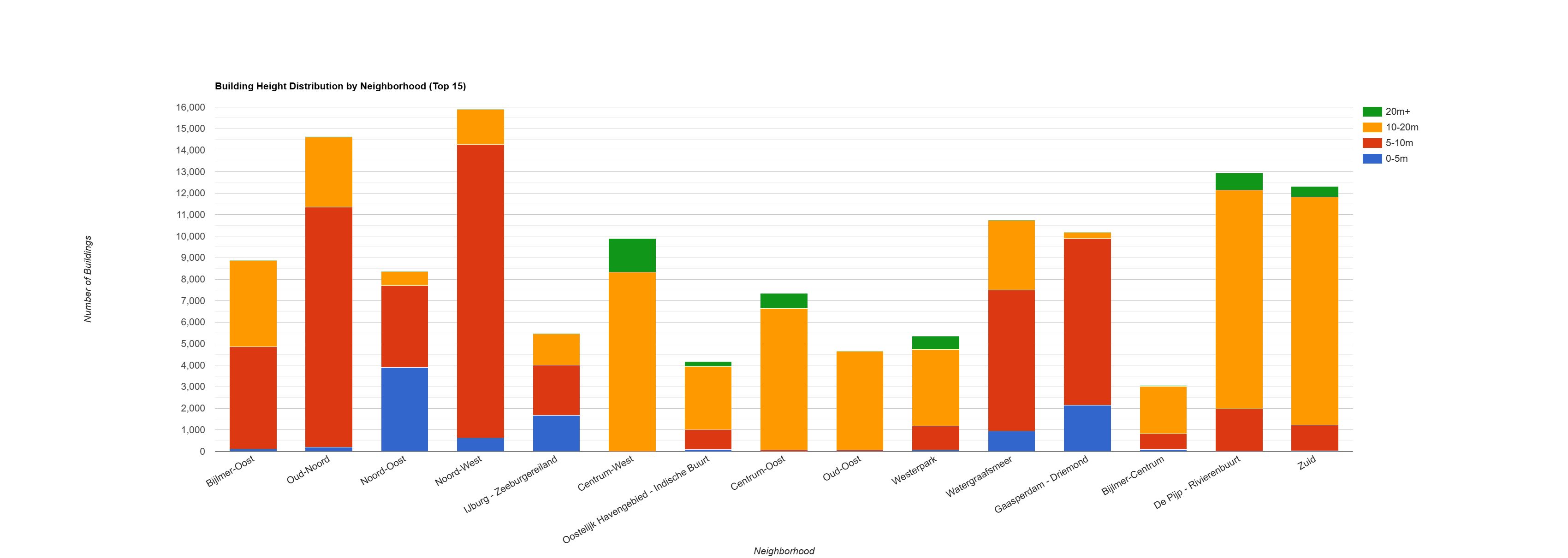
Building Height Distribution: There is a clear spatial variation in building heights. Neighborhoods like Bijlmer-Centrum and Bijlmer-Oost have a substantial stock of taller buildings, with a large number of structures in the 10-20m and 20m+ categories. This aligns with the known post-war development of high-rise residential blocks in these areas. Conversely, many other neighborhoods are predominantly low-rise, with the majority of buildings falling into the 0-5m and 5-10m height categories.

ghs_obat_layers_ht

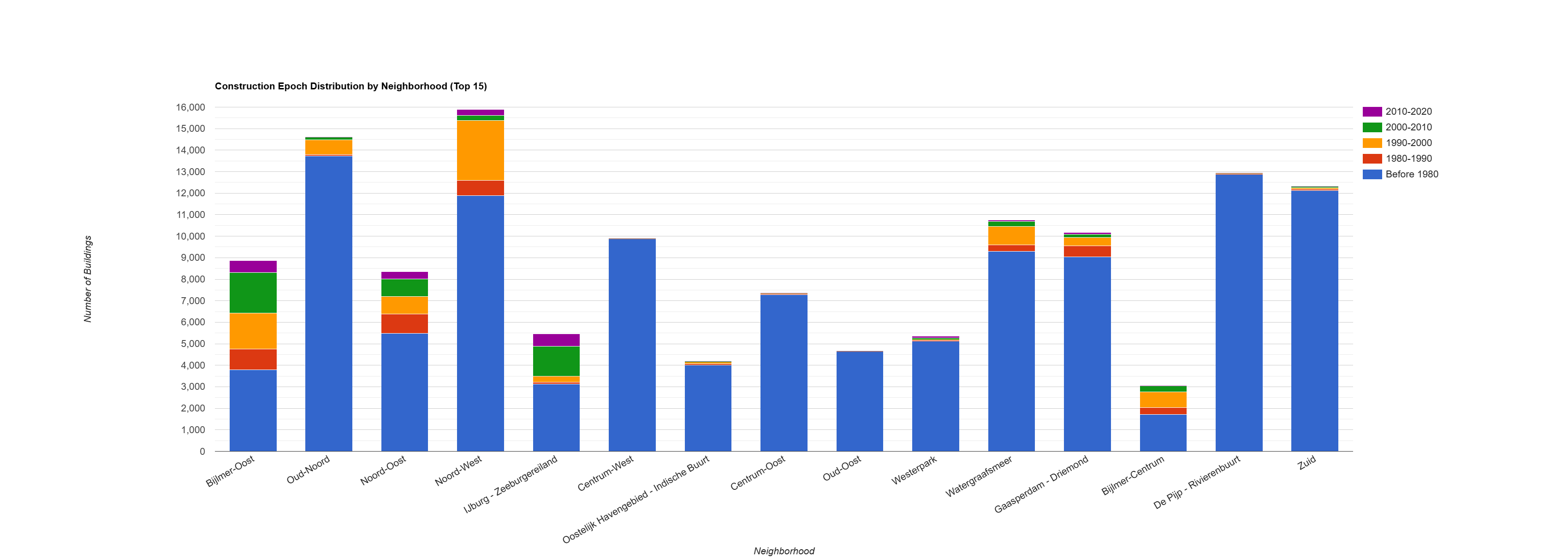
Mixed-Age Neighborhoods: Some neighborhoods, such as Watergraafsmeer, exhibit a more balanced mix of construction epochs. This suggests a history of continuous development and infill over several decades rather than a single, dominant period of construction.

These data-driven insights, derived entirely from Earth Engine, align with the known urban development history of Amsterdam and showcase how GHS-OBAT can be used for detailed urban studies.

5. Conclusion¶

This workflow provides a robust template for leveraging the GHS-OBAT dataset for sub-national analysis. It can be readily adapted to other cities, administrative boundaries, or to analyze other building attributes like functional use or shapefactor. The enriched feature collection can also be exported using Export.table.toDrive for use in other data analysis softwares. You can find the overall code here

Forum

Ask AI